Neighbourhood operations and filtering

Both buffering and triangulation have introduced the notion of proximity, underlining the potential importance of relationships between objects in space, between neighbours. Tobler's first law of geography is that: ``Everything is related to everything else, but near things are more related than others''. We will see that we can programme neighbourhood procedures by designing filters.

1. Neighbourhoods vector-style
   • Vector GIS with topological storage of geometric data already ``know'' about their neighbours. Typically, each arc in an arc-node structure will record the ID-number of the polygons on its left and right.

   • Consequently, asking questions like ``Find the sum of the lengths of the boundaries between residential and pasture categories in the land cover map layer'' is uncomplicated.

   • The same applies to making lists of neighbours: ``Make a list of all the owners of properties neighbouring schools in the north west of the city'', where neighbouring is taken to mean sharing a boundary in a cadastral map layer. The correctness of the list does however depend on the list of owners being up-to-date, being linked to the correct property ID's, and on the precision of the cadastral map layer.

   • Distance relations are more of a problem, because the system will typically find every object within the specified distance before going back to the database to check whether attribute conditions are fulfilled.

2. Buffers and neighbourhoods
   • In the raster case, the objects ``know'' nothing about their neighbours -- the ``knowledge'' is simply part of the grid system, and has to be reconstructed each time it is needed. On the other hand, it is regular and uncomplicated.

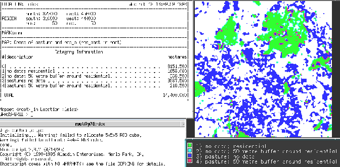
   • The procedures we have already learnt permit us to answer questions like ``Find the sum of the lengths of the boundaries between residential and pasture categories in the land cover map layer'', even though we have no topological measure of the category polygons.

   • One approach is to buffer one of the two categories out by one grid cell. If we then overlay the resulting map over the other category and cross-tabulate, we will find a category with a cell count approximating the boundary between the categories.

   • Naturally, the result will not be precise, but it is unlikely in the first place that metre-precision is a realistic expectation -- this is a typically ``fuzzy'' topic.

     Figure 6: Pasture land use category overlay over residential land use buffered by one cell.

     

3. Filtering and neighbourhoods
   • Filtering is a way of approaching data that comes from modifying unidirectional series, most often in time. In many cases it makes sense to compare results now with results from a comparable month or season previously, rather than with those immediately before. Spatial filters are different because they move simultaneously in two directions across the plane; they are 2D filters.

   • Filtering is much used in processing remotely sensed data, in order to reduce technical imperfections, and to enhance image quality. In vector GIS, filtering is difficult to handle, but in raster systems, it is simply another way of doing overlays.

   • If we start with a 3x3 filter, there are 9 positions: the cell itself, and its 8 neigbours to the N, NE, E, SE, S, SW, W, and NW. Overlay as we know it applies to the cell itself. Using filtering just diplaces the layer in the cardinal direction of the neighbour being processed. Remember that there is no data beyond the edges of the layer.

   • Say we expect the value of each cell to be the average of its neighbours. We can design a filter to calculate this as a little table, using map algebra multiplication. Here is the GRASS filter for ``rook's'' average:

     
     TITLE 3x3 rook's move
     MATRIX 3
     0 1 0
     1 0 1
     0 1 0
     DIVISOR 0
     TYPE P
     

     This can be used to compute expected values for cells, in this case a measure of spatial autocorrelation -- a measure of smoothness in this case.

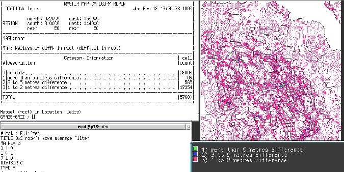
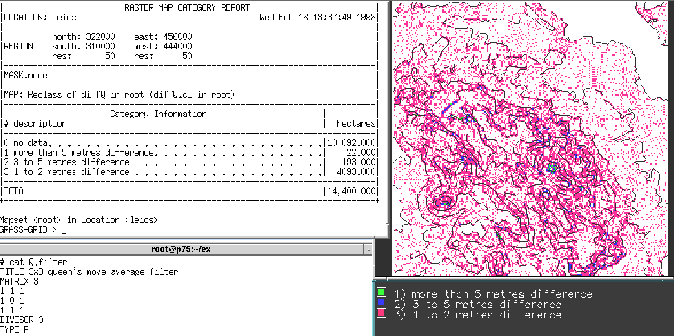
     Figure 7: Differences between elevations and estimated expected elevations, using the rooks' case filter.

     

     Figure 8: Differences between elevations and estimated expected elevations, using the queens' case filter.

     

4. Programming a slope filter
   • Before we move further to discuss surfaces, it may be helpful to see how powerful filters can be. The do not have to just be 3x3, and can be much larger, if the processes hypothesised have a larger range. For our present purposes we will keep to 3x3. We only have a simple raster GIS, which does not have a ``slope'' or ``gradient'' operation, but does filter, because filter is just overlay with displacement.

   • A standard method of estimating slope is to fit a 2D plane though the 9 cells in a 3x3 neighbourhood; Chrisman gives the details on p. 166. This describes the same algorithm as Map Factory presents (module reference p. 118).

   • The filters we need are for the two dimensions, X:

     
     TITLE 3x3 Sobel x filter
     MATRIX 3
     -1 0 1
     -2 0 2
     -1 0 1
     DIVISOR 8
     TYPE P
     

     and Y:

     
     TITLE 3x3 Sobel y filter
     MATRIX 3
     -1 -2 -1
     0 0 0
     1 2 1
     DIVISOR 8
     TYPE P
     

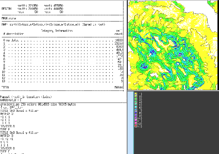
   • Running the following pseudo-code (like a script) gives us a layer with slopes in degrees (after cleaning up edge effects):

     
     slope.in.x = Filter elevation using "Sobel x filter";
     slope.in.y = Filter elevation using "Sobel y filter";
     slope = sqrt((slope.in.x ^ 2) + (slope.in.y ^ 2));
     

   Figure 9: Application of the slope filter to elevation data.