Continuous spatial variables
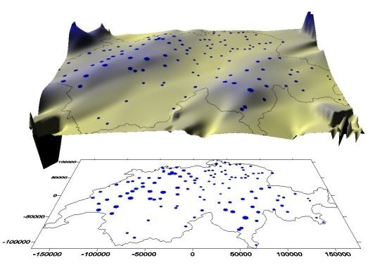
 Precipitation surface of Switzerland - Niederschlagsoberfläche der Schweiz (oben), Karte der Messstationen (unten)
The figure shows a precipitation surface of Switzerland: the blue dots represent monitoring stations; their size corresponds to the amount of rainfall at that station. The different heights of the surface and their color are associated with rainfall as well. The issues addressed in this lesson are:
- How can we construct a continuous surface from approx. 100 monitoring stations?
- Which tool can help us do this?
- What knowledge is necessary and which methods exist?
What do we mean by ''continuous spatial variables''?
In our example, rainfall is the variable. Let's perform a thought experiment: Imagine you could measure rainfall on any position along a route. You would have a spatially continuous measurement. Adjacent measurements would be either identical or vary only slightly (according to your definition of "neighborhood"). You may argue that precipitation often shows very well defined boundaries – and you're right. The "continuum of precipitation" is not mathematically perfect. Another example of a spatially continuous variable is sea level. However, virtually every natural spatially continuous phenomenon is subject to certain random fluctuations. Therefore, they can hardly be described in a mathematically perfect way (e.g. a function that exactly describes the rise of a slope, the distribution of different soil pH levels, or rainfall, etc.).
Random Function
From statistics we know deterministic (i.e. exactly predictable and mathematically recordable) and stochastic (i.e. purely random, unpredictable) phenomena. An example for a deterministic phenomenon is the fall of an object: we can calculate in advance the position of the object along the slope line at any point in time. In contrast, rolling dice is a purely stochastic phenomenon. In spatial analysis, we find phenomena that fall between deterministic and stochastic. They are referred to as random functions. Let's do another thought experiment: take a look at the flash-animation below. The points represent measurements of height. The actual heights between the measurement points follow a function that we do not know. However, we will assume that the heights of the unknown profile are not just random but are similar to the known adjacent points. Let's create a profile along the blue dashed line. In other words, we define a linear function between the measurement points. The red solid line shows the actual height profile. In the last image you can see a comparison of both profile lines. The height in this example is a random function – it is neither exactly mathematically recordable nor purely coincidental!
Please note: although the grid spacing is actually using discrete spatial units, continuous spatial variables are generally better suited to a raster model.
Learning Objectives
- You can describe the main types of spatial sampling.
- You can provide information about the reasonable size of spatial samples.
- You have mastered the basics of explorative variography.
- You can explain why knowledge of spatial dependencies is important for the analysis of continuous variables.
- You know the fundamentals of spatial estimation methods (interpolation).
- You can reasonably name applications for interpolations.
